Why Neural Networks are better than the old Banister/TSS model at predicting athletic performance.
Alan Couzens, M.Sc.(Sports Science)
July 26, 2018
I received a lot of follow up qu’s/discussion from this tweet on how I’m seeing Neural Networks consistently out-perform the Banister model (the model behind Training Peaks' Performance Management Chart) as a performance predictor for the vast majority of athletes....
Tough to ignore the numbers. For 13 of 15 athletes I looked at, a simple single hidden layer #NeuralNetwork provides a much better predictive performance model than the old Bannister/TSS model. Especially for high fitness athletes. pic.twitter.com/cLEl5h4cQJ
— Alan Couzens (@Alan_Couzens) July 7, 2018
So, I figured I would expand a bit and offer some thoughts on why the Neural Network looks to be a much better model for predicting athletic performance than the old (1975) Banister/TSS model here...
As the tweet suggests, for 13 of the 15 athletes whose long term data that I looked at, I could get a significantly better model fit to actual fitness (in this case athlete E.F.) by using a very simple single layer neural network vs using the prevailing Bannister/TSS model.
The neural network really separated itself at the individual level. While the group NN model was only slightly better than the group bannister model, it was much better able to describe load-performance relationships at the individual level. Given the importance of individualizing training plans, this is clearly a significant strength!
Interestingly, the 2 athletes who the NN didn't perform well for are the lowest fitness of the group (VO2max in the low 50's). Most of the remainder of the group have VO2max numbers in the 65 to 80 range (high level AGers and elites/professionals). So it seems that the neural net model might perform especially well in the case of higher fitness athletes.…
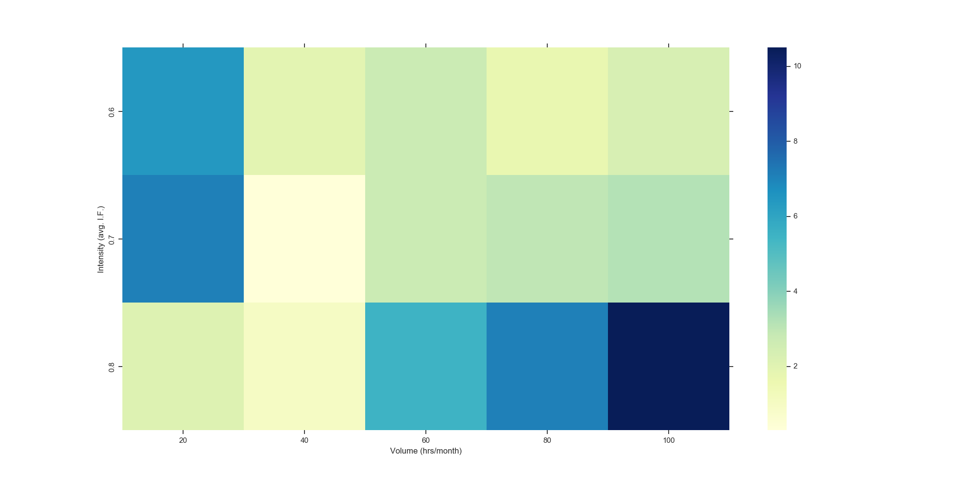
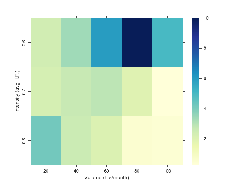
I dove into that question of who the Neural Network works especially well for with the above heat maps that show the error in prediction (RMSE) for the banister model (on the left) and the neural network model (on the right) for different levels of volume and intensity. While the banister heat map is darker overall (indicating higher error rates than the NN heat map), it is clear to see that especially for the higher level athletes – athletes training more than 60hrs/month at moderate-high intensities, the squares in the South East corner on the Banister model are much darker than those on the Neural Network, indicating a much higher error for this particular sub-sample. For these athletes, the Banister model significantly & consistently over-predicts performance for a given training load.
These clear differences beg the question... How do Neural Networks manage to outperform the prevailing model by such a large magnitude?
First a quick recap of what a Neural Network is & how it works.. (via this awesome gif! :-)
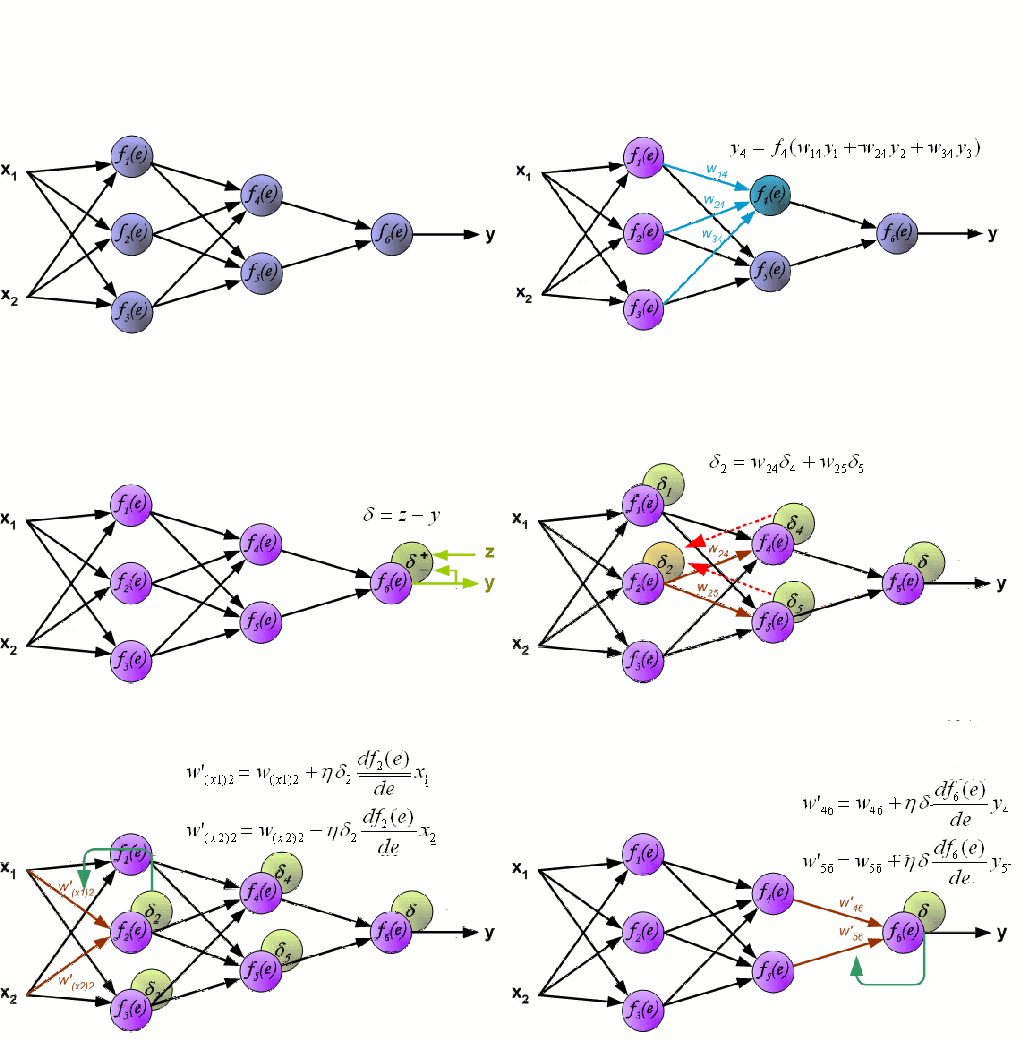
We have input variables (x1, x2) - for the purposes of this post, we could consider x1=fitness and x2=fatigue. We multiply each of these input variables by random weights (w) and pass the resulting equation down the network to a non-linear 'activation function' (f(e)). The outputs from the non-linear function on this layer -- f(random_weight1*input_variable1 + random_weight2*input_variable2...) are then weighted and passed down to the non-linear function in the next layer and so on, so forth. This process is repeated for however many layers are in the network & all of these neurons feed into one or more prediction neurons in the final layer of the network (y). In our case, Performance. Of course, because the initial weights were entirely random, the initial prediction will be very wrong! :-) so the network uses a bit of calculus to approximate where it went wrong at each step and 'back propogates' these errors back through the network to see which neuron's weights need to be adjusted and by how much. This process is repeated until the network is 'tuned' to the problem and is able to make correct predictions.
There are 2 main reasons that I think the NN is such a good fit to predicting performance in endurance sports, especially for higher level athletes
- As I’ve written about previously, a neural network (or really any modern machine learning algorithm) allows us to consider the impact of features separately, i.e. (given sufficient data) that initial layer of the network can have a whole bunch of variables (x1, x2, x3...) The Banister model is a much simpler input->output model that requires volume and intensity to be wrapped up into one variable. In the case of the original model, it has only 1 'x' input variable – TRIMP, in the case of the Coggan adaptation of the model – TSS. The big problem with this is that not all training load is created equally! 100TSS accrued as 4hrs of 'noodling' at 25TSS/hr is not the same as 100TSS accrued as an hour at threshold and yet, in this model, they result in the same predicted bump in performance! This issue was expressed succinctly in a 2006 critical review of the Banister model by Hellard et al..
"The nature of the immediate and long-term training effects of different exercises on the organism are so diverse that grouping them together or considering them as making up one single training stimulus would be unrealistic. A similar overall training load may correspond to two very different types of training. (There is a compensation in training volume in each intensity level). Accordingly, Taha and Thomas (2003) argued that the Banister model implicitly assumed that the performance activity matches the training activity and therefore does not consider the specificity of training."
It is unsurprising, then that a model that actually looks at the volume and intensity of training separately as independent contributors to performance is going to outperform a model that attempts to wrap them into one.
- While the above separation of features is a common trait of any modern machine learning algorithm, the Neural Network really shines in one very important way when it comes to performance prediction – it is able to reflect non-linear relationships between variables. The Banister model is tricky because when you look at it, you see exponents so it doesn’t, at first glance, look like a linear model. However, these exponents only reflect the decay of fitness and fatigue over time. If we keep these exponents constant, the model becomes 100% plain old linear regression…

The Banister formula is simpler than it looks. It simply says that the performance at a given time (Pt) equals the athlete’s initial performance level (P0) plus the accumulated fitness at that time minus the accumulated fatigue at that time.
If the fitness and fatigue constants (tau a/f) are truly kept constant (i.e. the model is time invariant), it essentially says that performance at any point in time is the direct summation of fitness - fatigue. In this sense, for a given athlete, if we increase CTL from 0 to 10, at the same level of fatigue, it should result in the same performance ‘bump’ as if you increase CTL from 100 to 110. In practice, any experienced coach knows that this isn’t the case and that as an athlete gets fitter, performance gains are harder and harder to come by. The Banister model is not able to reflect this reality. This limitation of the Banister model was also noted in the Hellard study referenced above..
"In the Banister model, training impulses are proportional to the training loads then, greater loads induce more fitness and fatigue acquisition. But previous studies reported that the impact of training loads on performance may have an upper limit above which training does not elicit further adaptation of the organism (Fry et al., 1992; Morton, 1997); Additionally, the procedure assumes the parameters remain constant over time, an assumption that is not consistent with observed time-dependent alterations in responses to training (Busso et al., 1997; Avalos et al., 2003; Busso, 2003)."
So what's the solution?
The Neural Network, of form...
ŷ=relu(ΣWiXi+b)
(where W is the applied weight, X is the feature matrix, b is a bias factor and i is the number of neurons in the hidden layer of the network) OR in Banister terms..
pt=relu(ΣkaiWi-kfiWi+p0)
...while equally simple to express, (or even simpler to implement in code..)
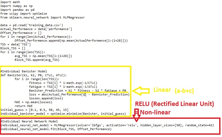
...has a distinct advantage: Because the whole formula passes through a non-linear function, in this case - a Rectified Linear Unit (ReLU), as the chart below shows, by rectifying our linear restriction we can make our performance model ‘bendy’....
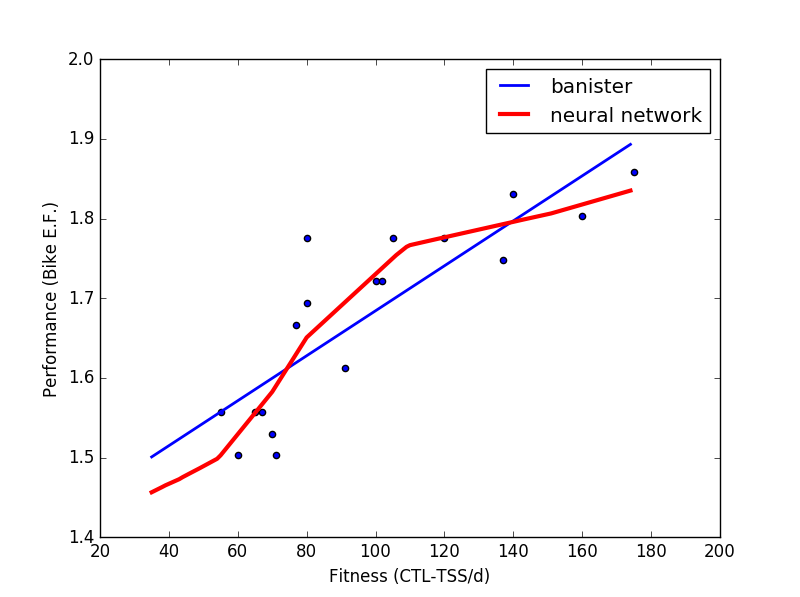
In more ‘math geek’ terms, the Neural Network is a model that is able to accommodate non-linear relationships between the variables, e.g. the diminishing returns from training load as performance increases that the Banister model cannot.
Above you’ll see this non-linearity on display with 2 seasons worth of data for an elite triathlete that I work with (peak E.F. 1.87). Fitness (in this case CTL) is shown on the x axis and the changes in the athlete’s Performance in this case bike 'Efficiency Factor' (Power/Heart Rate) is shown on the y axis. I only included points that ended with fatigue~=fitness (i.e. no taper/unload blocks) so that we could easily visualize it as a 2 factor model by keeping the fatigue aspect of the model constant.
You can clearly see that the athlete’s performance ‘bump’ for a given bump in chronic training load is not constant but varies in accordance with how ‘far along’ their fitness already is. I.e. a 20 CTL jump in fitness from 140 to 160 CTL gives a lot less E.F. improvement than the same 20 CTL jump from 80 to 100. This relationship is shown in the table below.
| CTL | Neural Net Predicted E.F. | Bannister Predicted E.F. |
|---|---|---|
| 50 | 1.49 | 1.55 |
| 100 | 1.73 (+0.24) | 1.69 (+0.14) |
| 150 | 1.80 (+0.07) | 1.83 (+0.14) |
| 200 | 1.85 (+0.05) | 1.97 (+0.14) |
The Banister model has a hard time reflecting this and predicts the same jump in performance for each jump in CTL/Fitness, while the more complex Neural Network can easily model the reality of diminishing returns. This inherently high 'bias' of the Banister model is what leads to Banister over-predicting performance for high level athletes in the heat maps above.
Bottom line: A good performance model for high level athletes needs to be able to bend!
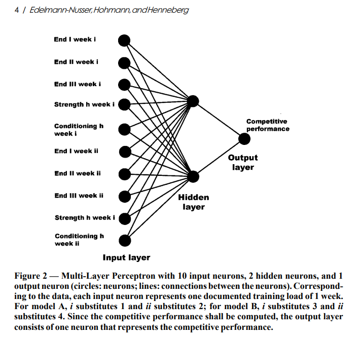
And I'm not the first to see the superiority of a 'bendy' model like a neural network to performance prediction in athletes. Edelmann-Nusser et al. (2002) used the following basic neural network to model the performances of an Olympic backstroker in the lead up to the 2000 Olympics and were able to use the model to predict performance within 5/100's of a second!
But this 'bendiness' comes at a price...
The problem of 'Over-fitting'
In the immortal words of Spiderman :-)...

A neural network is so powerful that, given enough neurons, a simple single layer network can approximate any non-linear function. Think about that for a sec, if I give it a circle, it can learn a circle. If I give it a picture of your head, it can learn your head :-) Given this flexibility, how do we know that the network is truly learning generalizable patterns in our data vs just 're-drawing' our data? Simple: We sit it down at the proverbial school desk & test it! We hold back a portion of our data and after the network has built the model, we feed it this 'holdout set' and see what it predicts. If the network predictions line up with reality, we can say it has 'learned' the underlying patterns in the data and, congratulations, we have a good predictive model!
But what if we don't have a good predictive model? What if our model has 'overfit' and the fit of our test set is way off reality?
The flexibility of the neural network comes into play again. There are a number of 'knobs' we can tune within the network to improve the power of our model - lots of complicated stuff, like the alpha regularization parameter, the learning rate, the momentum & even the type of non-linear activation function we choose. We can also restrict the epochs, i.e. cut back the time that we let the model train on the data. But, if we see that our model is overfitting the data, the most simple (& powerful) change we can make is to just simplify the architecture of the model. In a model that over-fits, it is generally the case that the model is too complex for the amount of data we have so, in the absence of having more data to feed it, what do we do? We simplify the model!
In this day and age of thousand layer 'deep learning' nets it can be easy to forget the power of a really simple single layer, 'couple of neuron' networklike the one used in the Edelmann-Nusser study above. Given the reality of that curvilinear pattern of 'diminishing returns' between load and performance that we talked about above, 9 times out of 10, when it comes to modeling athletic performance any model that can bend is going to beat a linear model (like Banister's) and it only takes one neuron containing a non-linear function to give us a model that can bend!
For example, here is the same data passed through one single, solitary tan-h neuron - about as simple as a neural net can get(!) & still obviously a better fit to the data than the linear Banister model!
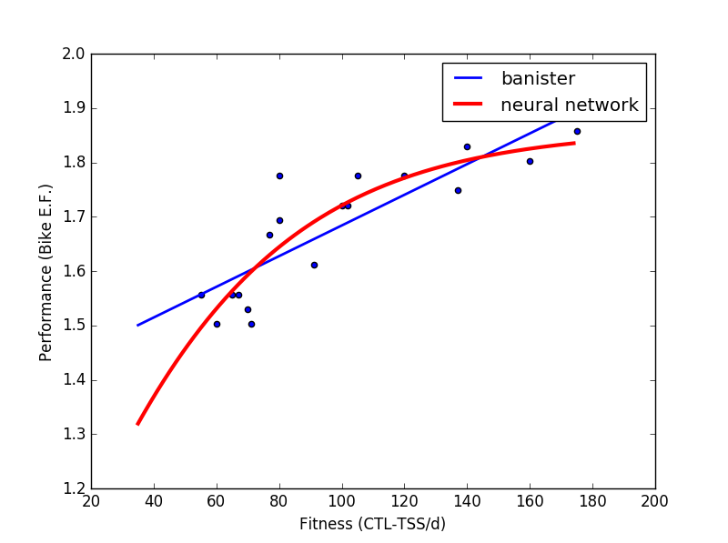
So, in practice, if we only have a limited number of training blocks for a new athlete, and our model is way over-fitting the data, the simple solution is to chop it down until it doesn't. Cut back the number of neurons in the network until that validation score comes up. As I said, in our particular case of dealing with data that shows a consistent pattern of diminishing returns, even one non-linear neuron will beat out a linear model most of the time!
As an aside, if you're working with Python's Scikit-learn library, its 'grid-search' function will test out these structures for you and come back with the one that gives the best validation score on your data.
####
The Excel savvy among you might be thinking, isn’t all of this Neural Network stuff overkill? I could reflect the above 'bend' pretty well with a simple logarithmic regression? And you’re right. In this case you could, but not all athletes have the same shape of curve. For some athletes, the relationship is more linear (for those athletes in my sample who had a decent fit with the Banister model). For some athletes, the shape of the relationship may be even more of a ‘dog leg’ with a fairly linear relationship up to a point followed by a plateau as the limits of time and energy are pushed. For others still, the relationship might be an ‘inverted U’ where performance actually starts to decline as we overdo things with the training load. To reflect all of these individual possibilities, we need a non-parametric model, a model without a lot of prior assumptions that is flexible enough to handle all of the above potential dose-response relationships & that is why the Neural Network is so powerful in its ability to reflect very individual dose-response curves.
In summary, when it comes to understanding the dose-response relationship for a given athlete, a neural network opens up another dimension in its ability to look at the impact of volume and intensity as separate entities and its ability to assess how fitness changes (non-linearly) at different levels of load. For these reasons, it is quickly becoming my ‘model of choice’ when planning the long term training 'dose’ to achieve a given level of performance.
Train Smart,
AC
