Python for Coaches Part 2: Getting hrv data from fit files

In my last post,, I aimed to gently introduce Python to sport scientists and coaches in a functional way - by using Python's fitparse package to extract data from fit files. I know that, at the end of the post, I said that my follow up would be how to extract long term data from multiple files in a folder but I received a question that I thought it would be useful addressing first....
So, how do I get heart rate variability data from this file?
As you probably know by now, I am a huge fan of using heart rate variability to guide the training. And, while there are many app options available to collect your data, it can also be useful to know how to pull heart rate variability data straight from your Garmin's fit file.
For starters, many athletes already have a Garmin watch of some sort so this provides an easy entry into the world of HRV monitoring without having to purchase any additional hardware or software.
But, maybe more importantly, using Python to understand your data on a deeper level gives the coach more flexibility over the metrics that are being collected & also gives greater visibility into how heart rate variability is being calculated and whether the numbers that you're seeing are sufficiently accurate for that individual to be considered useful.
Most of the HRV apps offer limited visibility into what is actually going on 'behind the scenes' at the beat to beat level. Python can definitely help with this!
So, let's get started pulling heart rate variability from one of your plain old fit files..
A quick note before we begin that, just like the last tutorial, I've built an interactive Colab workbook for this tutorial that you can save a copy of and play with, with your own data. Simply upload your own fit file to the workbook (to the folder in the left menu), rename it to 'my_hrv_file.fit' & you will be able to run the cells with your own data. Remember that each cell must run sequentially so if you get an error, be sure that you've hit the 'play button' in the top left corner of each cell before it. OK, so on to the fun of diving into your heart rate variability data!
The first step is making sure that your watch is configured to record HRV data! On newer watches, this is simply a matter of turning the function on! If you go Settings->Physiological Metrics->Log HRV & turn the toggle to "on" (as the pic below illustrates) you're good to go!

If you have an older watch (920 XT, Fenix 3, Forerunner 620 etc) you will need to install a special file that enables HRV recording to the "NEWFILES" folder on your watch. You can find a copy of the file (enable_hrv_settings) in my github repo Just plug your watch into your computer and navigate the the NEWFILES folder and drop the file in. Other than that, make sure your watch is set to one second (not 'smart') recording and you'll be good to go!
Now that we have the watch configured, you're set up to pull HRV from any fit file. So, let's do that...
!pip install fitparse
from fitparse import FitFile

fit_file = FitFile('my_hrv_file.fit')
Just like the last blog, we kick things off by importing Python's 'fitparse' library - a package that specializes in parsing the data from Garmin's fit files.
However, you'll probably remember that when we did that last time, we iterated through the files 'record' messages & we didn't see any HRV data, so where does the HRV data live?
Conveniently, it lives in a message named 'hrv' :) So, let's access this info...
for record in fit_file.get_messages('hrv'):
        for record_data in record:
          print(record_data)
If you run the above cell, you'll see that a bunch of numbers in groups of 5 shows up. So, what does this all mean? What HRV data are we looking at?
Each of the tuples (a 'tuple' in python is just an unchangeable list of values between 2 brackets) represents the RR intervals from one second of sampling. There are 5 values because, by turning on HRV mode, we tell our watch to sample 5x per second. In the case of a resting test, most of these values will be 'None' because one sample per second (60 samples per minute) should be about all we need.
So, what do I mean by RR interval? RR interval is the core unit for any HRV calculation and represents the time (in this case, in seconds) between each R 'spike' on an ECG...

The crux of all HRV calculations is measuring how variable these time frames between the R waves are.
Since this is our starting point for all calculations, let's start by pulling all of these RR intervals from our tuples into a single list that we can reference later...
RRs = []
for record in fit_file.get_messages('hrv'):
        for record_data in record:
          for RR_interval in record_data.value:
            if RR_interval is not None:
              RRs.append(RR_interval)


print(RRs)
Most of the above should be familiar from the last blog. We created an empty list called RRs to hold all of our RR intervals by coding RRs = []. Then we gave our loop a deeper iteration (you'll remember that the most indented blocks of code loop first). So, now we loop through messages named 'hrv' and we loop through each of those 5 item tuples that we looked at above. Finally, we add one of those 'if' conditionals in saying "if" the RR interval is not "None", i.e. that it's an actual number, let's add it to our list of RR's. If it is a "None" our loop will simply skip over it and not add it to our list. We finish up by printing out our nice, clean list of RR intervals from the file.
But just how 'clean' are they? Let's take a look. You'll remember from our last post we used matplotlib to visualize our data. Let's mix it up and use a different package this time - Plotly.
Plotly is my favorite data visualization tool. Largely because it plots interactive plots by default (if you're following along in Colab, you'll notice if you hover over the plot, it will display tooltip data from each point) and it also has a javascript version which makes it really easy to display your python data on a web page. So let's start by installing...
!pip install plotly
Looks like it's already in Colab. Cool. Now let's plot our RR interval data.
import plotly.graph_objects as go

x = []
total = 0
for i in range(len(RRs)):
  total = total+RRs[i]
  x.append(total)

fig = go.Figure(data=go.Scatter(x=x, y=RRs))
fig.show()
Let's go over what we did in the code above...
First we imported the long named plotly package and decided to just call it 'go'
We then set up an empty list for our x values (since we'll need those to tell our chart where to plot). Then we do something kind of interesting with the 'total'...
For the x axis, each beat isn't occuring at a 1s interval so we can't just increment by 1s. Instead, the time on the x axis will be the sum of all of the RR intervals leading up to that point so that's what we do with the total. We just keep adding each subsequent RR interval to the 'total' to get the total time that has passed when each beat happens & then we append that to our list so we get a list of the duration when each beat occurred as our x axis.
Then we build a figure, telling our go library that we want a scatter (aka line) graph and our data is our x values (duration of the test) and our y values (RR interval).
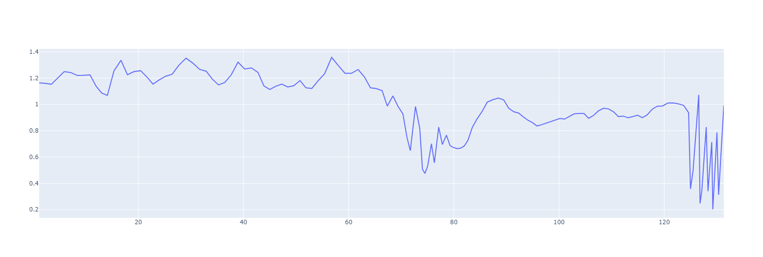
When we plot our chart, the advantage of being able to visualize our data really starts to show...
So what do you see when you look at the chart?
First thing that you'll probably notice is that there is some weirdness happening at about the 60s mark. All of a sudden the RR interval drops a lot (i.e. the heart speeds up) & it becomes a lot more variable (lines become squiggly) before stabilizing. What's going on here?
Well, for the last 20 years or so, even before I started recording HRV, I have done a standard morning recovery test - 1 minute supine, followed by 1 minute standing. Initially, all I tracked was the difference in HR between the supine and standing position (a useful metric in itself!) but for the past 12 years or so, I added pure HRV to that. Now, as you can see, HRV changes depending on whether I'm supine or standing so, to calculate our metrics, we're going to want to filter out one or the other. Let's do that in a bit...
The other thing that you probably notice is that, there are some periods in there where things go 'spiky'. In the case of this file, they happen on the transition from supine to standing and at the end of the test. Odd spiky beats are actually quite common and need to be filtered out to give us accurate numbers. These can come from interference on the monitor, or from ectopic beats caused by some faulty wiring in the heart. These pre-atrial and pre-ventricular contractions are quite common as single weird beats. It's a little less common to see lots of weird beats strung together like at the end of my file. This is because I have a heart condition - atrial fibrillation that, at times, leads to faulty electrical signaling in the heart. Clearly this is abnormal and we don't want to include the weird beats in our file. So, let's first filter them out...
filtered_RRs = []
for i in range(len(RRs)):
  if RRs[(i-1)]*0.75 < RRs[i] < RRs[(i-1)]*1.25:
    filtered_RRs.append(RRs[i])

print(filtered_RRs)
So, to filter out the beats caused by my 'dicky ticker', we simply built a list of filtered RR intervals and we only added RR data to the list if it didn't differ from the previous beat (in either direction) by more than 25%.
This is generally a pretty safe number. If we think about normal SDNN numbers, i.e. the standard deviation between beats, an average athletic number might be somewhere around ~100ms. If the average heart rate is 60bpm, that's an RR interval of 1000ms, so if a beat differed from the last by 250ms (25%) of the RR, it would be pretty unusual when the standard dev is 100ms. If normally distributed, we'd expect this to occur less than 5% of the time. However, if we see an individual with very high SDNN of, say, 200ms, that difference between the 200 and the 250 starts to dwindle and we could end up eliminating a lot of healthy beats if too aggressive with our filter. Another reason that it is great to be able to use Python to visualize the raw data to see what looks like normal variability vs weirdness!
In our case, we don't know my SDNN (yet :) but let's have another look at the data to see if it eliminated the spiky beats, using the same code that we used above (only this time for filtered_RRs)...
import plotly.graph_objects as go

x = []
total = 0
for i in range(len(filtered_RRs)):
  total = total+filtered_RRs[i]
  x.append(total)

fig = go.Figure(data=go.Scatter(x=x, y=filtered_RRs))
fig.show()
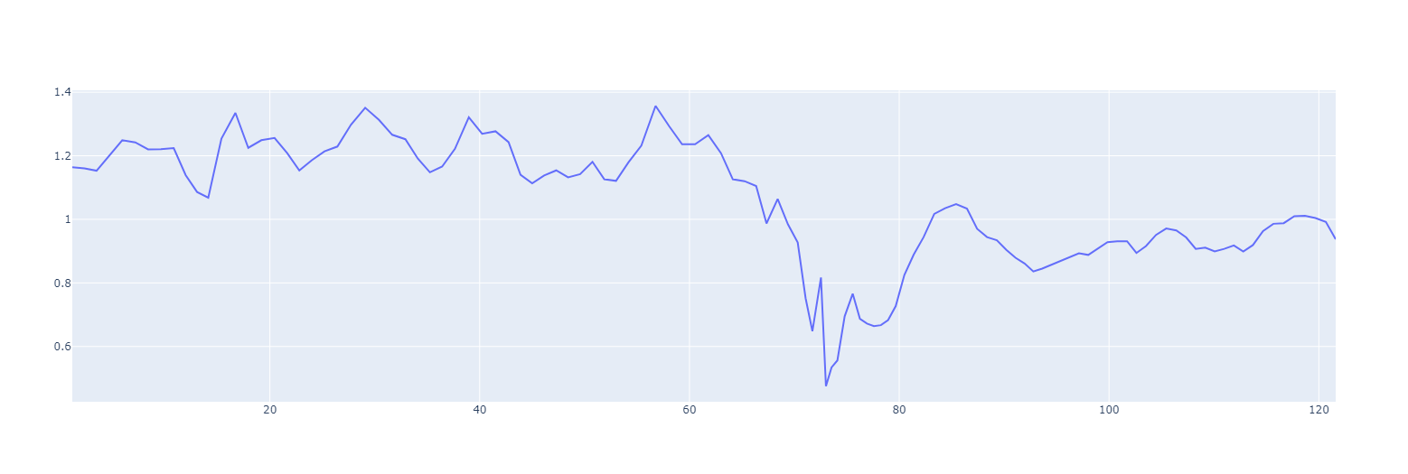
Much better! Importantly, the normal variability that we saw in the previous plot remains but the vast majority of the spiky beats are gone!
Now let's go back to my first problem of not budging on my test protocol :-) We only really want the first 60s (supine) portion for the HRV calculations so let's do that...
laying_down_bit = []
totals = 0
for i in range(len(filtered_RRs)):
  totals = totals + filtered_RRs[i]
  if totals < 60:
    laying_down_bit.append(filtered_RRs[i])

print(laying_down_bit)
Here we use the same 'totals' approach that we used above to simply build a new list that only includes RR intervals up to a total test duration of 60s, i.e. the supine bit of the test.
Looks like it did the job. Our list is much shorter now but let's visualize it to make sure. Actually, since we keep coming back to the same block of code, just with a different list, to visualize our plot, now would be a good time to introduce functions.
Conveniently, a function is just a re-usable block of code that we can pass changing variables to and it will return a different result depending on what we pass. It is defined in Python by writing "def", i.e. define my function. Let's build one for our plots that we can re-use if we need to plot further lists...
def plot_my_list(my_list):
  x = []
  total = 0
  for i in range(len(my_list)):
    total = total+my_list[i]
    x.append(total)
  fig = go.Figure(data=go.Scatter(x=x, y=my_list))
  fig.show()

plot_my_list(laying_down_bit)
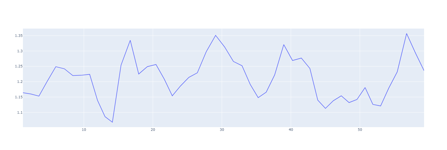
Excellent! Worked like a charm! We defined our function by coding def plot_my_list(my_list) and then called it by simply passing the 'laying_down_bit' of the data that we split off above to it by typing
plot_my_list(laying_down_bit)
and the function did its job and just plotted the first 60s of our clean, filtered data. As you can see, even with the filtering, there is still plenty of variability at play with the time between beats varying between ~1.05s to ~1.35s largely in coordination with my breathing.
Our next step is to calculate some of the common HRV metrics from this data. Actually, we need to do one more thing before we do that. The standard unit for HRV metrics is milliseconds (ms) but our RR intervals are still in seconds, so let's fix that. Are you ready for a new Python tool?
So, we could just use our standard loop to do that, right?
laying_down_bit_ms = []
for i in range(len(laying_down_bit)):
  laying_down_bit_ms.append(laying_down_bit[i] * 1000)

print(laying_down_bit_ms)
But a more succinct way of building a new list with a loop in Python is using a list comprehension. The list comprehension is simply a shortcut that lets you put your new list and the calculation that you're applying to the old list on one line. It simply goes...
new_list = [expression for item in old_list] Or, in our case...
laying_down_bit_ms = [RR_interval * 1000 for RR_interval in laying_down_bit]

print(laying_down_bit_ms)
There we go. Much more succinct. Everything we need in one line. The 2 tools that I introduced above, functions and list comprehensions will greatly improve your coding. Functions especially. Separating your code into well named blocks akin to paragraphs makes for much shorter, much more efficient, much more readable code. Highly recommended!
So now we have a list of 'clean' RR intervals in milliseconds for only the laying down portion of my test. Let's move on to the fun bit - calculating the common HRV metrics. Let's start with the easiest - SDNN.
SDNN is representative of the total power of the autonomic system, i.e. the combined power of the sympathetic ('fight or flight') and parasympathetic (recovery) systems., i.e. it is a good indicator of our ability to both do and recover from work. As such, it is a very important metric for the coach to know!
As we touched on earlier, mathematically, SDNN is simply the standard deviation of normal-normal beats, i.e. the standard deviation of our list after we remove spiky beats. Now that we've done that, it is ridiculously easy to calculate...
import numpy as np

SDNN = np.std(laying_down_bit_ms)
print(SDNN)
Easy peazy! We simply pulled in one of Python's most useful math libraries NumPy and called its standard deviation function on our list.
Now let's move on to the more commonly used and slightly trickier rMSSD...
rMSSD is representative of the strength of only the parasympathetic branch of the autonomic nervous system, i.e. it is a good indicator of our ability to recover from work. This is distinct from the athlete's ability to do work. By knowing both of these (SDNN & rMSSD) we can then better discern the difference between being ready to do work and the ability to recover from said work.
Mathematically, rMSSD is simply the root...mean...square of....successive differences so let's calculate those step by step, starting at the end with 'successive differences' and working our way back to 'root'...
successive_differences = [laying_down_bit_ms[i+1] - laying_down_bit_ms[i] for i in range(len(laying_down_bit_ms)-1)]

print(successive_differences)
So we used our new fangled list comprehension that we introduced above to loop through each item in our list of RR intervals and we subtracted the following beat from the current beat to get the 'successive difference'.
You'll notice that some are positive and some are negative. This can be confusing as we're not really interested in the direction of difference between successive beats, just the absolute amount so let's get rid of the minus sign by moving on to the next bit of rmSsd, i.e. squaring each of the values.
squared_successive_differences = [successive_difference**2 for successive_difference in successive_differences]

print(squared_successive_differences)
Now let's move onto the next letter - M for mean.
mean = np.mean(squared_successive_differences)

print(mean)
And the last letter - R for root.
rMSSD = mean**0.5

print(rMSSD)
The square root of a number is the same thing as the number to the power of 1/2 so that's what we did above with '**' python-speak for "to the power of" to get the root of the mean squared successive difference.
Budabing badaboom! We just calculated SDNN and rMSSD the long way straight from our HRV file! Specifically, in this case, SDNN = 68ms and rMSSD = 57ms.
Hopefully doing it the long way above helped to increase your understanding of both Python and of Heart Rate Variability and how some of the common metrics are calculated. I'll post a short script of all of the above in the Github repo so you can continue to play around with your own files.
In my next post (I promise, this time :-) I'll dive into how to pull bigger data over multiple seasons as the first step in building athlete specific predictive models.
Until then...
Train smart,
AC