Using machine learning to predict injuries - part 3:
The factors that best predict injury in endurance athletes

Alan Couzens, M.Sc. (Sports Science)

Jan 9th, 2017

In my last 2 posts (here & here), I introduced some basic machine learning concepts that I’ve found to be useful in analyzing and making sense of the mass of data created by athletes on a daily basis! I introduced you to the Scikit-Learn library and showed how with the use of some basic Python code we can import machine learning algorithms that make discovering relationships within your data & using these relationships to predict what will happen (given unseen data) a breeze.

I provided some simple snippets of Python code to illustrate the basics of this approach. We coded up a short numpy array of some sample data of various features (load, sleep, stress, training load ratio & BMI) along with a classification of injured v not injured to build a working model & then used that model to predict whether an athlete would become injured or not injured based on previously unseen data. In the real world, however, hand-coding all our data into scripts is laborious, unnecessary & very limiting in how much we can learn from the mass of data around us. But fear not! Python has some great tools that let the coach pull directly from the BIG(gish) data that can be found in databases or even simple Excel spreadsheets! Pulling in this information from external sources/files significantly increases the amount of data that we can learn from & significantly improves the predictive power of our models!

If you already have a database at work, this is as simple as running a standard query in python’s SQL alchemy library e.g.

...will pull all values from the respective columns in the database into Python lists that can then be fed directly to the numpy array.

But, even if working with a run of the mill .csv file (as found in Excel or the like) the process isn’t that much harder…

If you think, for a second, about the mass of data that is available in spreadsheets or as csv exports, you can sense the power of these few lines of code. Want to mine years of data from Training Peaks for insight? Simple – export it as csv, crank up your python editor and model whatever relationships you want!

But, back to our relationship of interest: The impact of various load and lifestyle factors on injury rates in athletes….

If you're a die hard rationalist, like me, who really wants to understand the inner workings of your model (as opposed to those pure empiricists who only care about building a model that serves as a good predictor - blah, where's the fun in that? :-), the best machine learning algorithm for the job is, arguably, a Decision Tree.

I don't like to play favorites when it comes to model selection but Decision Trees (& their variants) have a lot going for them both in terms of their power, their ease of use and, maybe more importantly, their understandability. They have a hard time with forecasting and therefore maybe aren't as useful when applied to performance modeling but in many instances, & especially classification problems (like injury prediction), they're tough to beat!

A decision tree is a super easy to understand model. We use them every day….

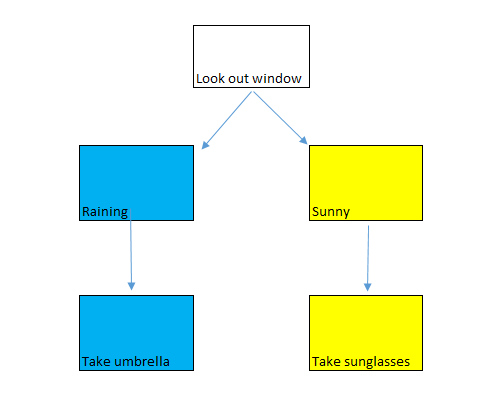
Or, in our context….

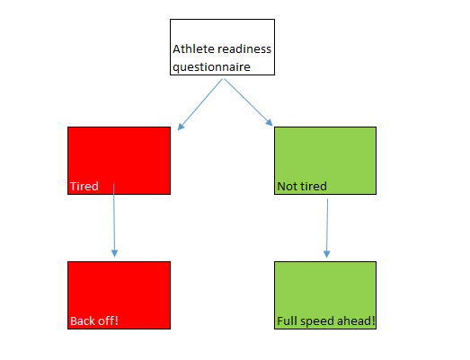
But with the computing power of our PC we can do much better. We can quantitatively define these features – how tired is too tired (that things are sufficiently 'risky' that we should 'back off' the training load)? And how do these forces work together, i.e. can I afford to be a bit more tired if I'm away at a training camp without the regular stress of normal daily life? Can I afford to be a bit more tired in the day if I have more time to sleep and recover at night? etc.

These complex weighing processes aren't a new feature of coaching, the same process occurs in the 'gut feels' of experienced coaches the world over! But now, thanks to the awesomeness of Python, the scikit-learn library has a powerful Decision Tree module that helps us visualize and systemize some of these 'inner weighings' to bring these factors into the open & speed up the learning process. This module is already built into the Scikit-learn library & it is extremely powerful in its ability to sift through all of the variables at play concurrently & it's just waiting to provide us with all kinds of insight on these relationships & the relative importance of each of the various input variables…

Here is a Python script that accesses that Decision Tree module to build an injury prediction Decision Tree using Scikit-Learn...

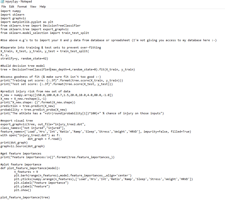
A quick summary of what the code is doing..

On the first 7 lines we import all the ‘stuff’ we need – numpy, sklearn, a couple of graph builders (graphviz & matplotlib) so we can visualize our tree & a chart of the various feature importance & a module from sklearn that splits our data into training and test sets so we make sure we don’t overfit (see below).

Then I insert a comment telling you that I'm not giving you access to my database :-) Data is gold in this day and age. This is where you would inser the code above to draw from your own data in a .csv file or database.

Then we separate our data into training and test sets with the train_test_split() function to prevent overfitting...

Overfitting is the greatest challenge of modern machine learning. With the power inherent in many of the models these days, it’s entirely possible to come up with a model that near perfectly fits the data. You could think about this on a scatterplot as a line that just connects all the dots – going from dot to dot rather than the typical trendline which provides a ‘best line of fit’ for the dots. With a simple linear model, like a scatterplot, this isn’t a prob, but the more sophisticated the model gets the finer that line between just describing the data vs coming up with a general pattern for the data becomes. The problem with going dot to dot is that, while it looks great for the current data, the ability of the line to generalize & predict future dots on the chart isn’t good. In order to produce a good model that does a good job of predicting future occurrences (the whole point of machine learning), we want general patterns rather than perfect descriptions. By keeping some of our data back as we build the model and then using it later to test how well it fits we can see how well our model generalizes to unseen data. That’s what we do on the next line – split our data into training and test sets with train_test_split

Then, with the simple command DecisionTreeClassifier().fit() -- we build our decision tree model with the training data.

Then, by applying tree.score() to both the training and test data we assess the 'fit', i.e. just how well our model predicts. We assess this on both the training data and also, more importantly, on the (unseen) test data because we want to make sure that our model does well on predicting data that it hasn't yet seen, i.e. we don't want to 'overfit' it to the training data as described above.

Training set score: 0.977

Test set score: 0.902

In this case, the model gives us ~90% classification accuracy on the test set. Not bad! You can see that there is still a significant difference between the test and the training set though, indicating that our model may still be a little 'overfit' to the training data, suggesting we may even be able to improve the model by simplifying the structure, i.e. 'pruning our decision tree' by chopping off a branch & changing that 'max depth' parameter to 3. Or we could implement an ensemble method like 'Random Forests', which, as the name suggests is made up of a bunch of independent decision 'Trees' all trained independently on the same data set.

Then, just for fun, we take the model for a test drive by using tree.predict(X_new) to ask the model to predict the incidence of injury for a new athlete (X_new) that the model hasn't yet 'met'..

We ask the model, based on the above inputs, will we have an injured athlete on our hands? And...

The athlete has an 83% chance of injury based on those inputs

No bueno! We might want to dial down the load on the basis of this!

Then, for the really neat stuff -- we export the model in visual form to give us further practical, actionable insight as to what's going on 'under the hood', i.e. what decision process is the model going through to determine whether an athlete is injured or uninjured and where do these key 'cut offs' lie? That's pretty much it!

When I hook this this script up to my database & run it for insight, it spits out the following charts that provide us with further insight on the various factors at play, their relative weights and how they all come together to lead to an injured or uninjured athlete…

Feature importance.

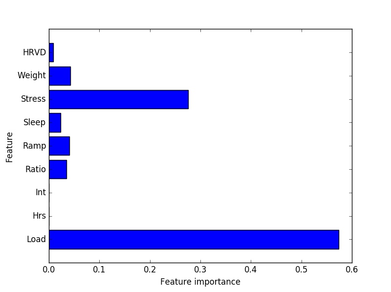
The decision tree will let us know graphically which variables(/'features') are most predictive(/important) in the model. It will also drop those features that don't add any additional predictive value to the model. You can see in this case, pure training load tops the list (by a good ways!). My data would suggest that athletes who train a lot (>125TSS/day) get injured far more frequently than those who don’t.To quantify, the injury rate of this group is more than 5x greater than the injury rate of my athletes averaging less than 125 TSS/d. Not exactly an earth shattering revelation but nevertheless an important one given the current interest in the importance of ratios over pure load. This data would not support that perspective.

The key message here is that the athlete has a limited 'shelf life' at very high loads. The time spent at the highest 'altitudes' of the peak must be planned carefully and must line up with the greater life as a whole.

This bring us to our next point...

Life stress, which my athletes monitor on a 1-5 scale, is a strong predictor of injury – periods of high stress tend to create a ripe environment for injury risk. This is especially true when combined with the high load above. For a high load athlete (>125TSS/d), if average daily stress is scored higher than 2.75/5, the incidence of injury goes up by a factor of ~10! This brings to mind the importance of a simple, stress free existence to handling high training loads &, more practically for us in the Western World, a realization that training stress and life stress must be in balance.

Additional factors: Ramp rates & weight. Athletes of higher weight in my sample (greater than 73kg) do tend have slightly higher injury rates than lighter athletes. Also, more aggressive ramp rates do tend to lead to higher rates of injury than a more gradual approach. Specifically, ramps of >16.5 CTL per month lead to a slightly greater incidence of injury in my sample.

In addition to the feature importance chart above, the code will actually produce a visual representation of the decision tree that shows those critical 'fork in the road' numbers that lead to injured athletes. This is shown below…

Injury prevention Decision Tree

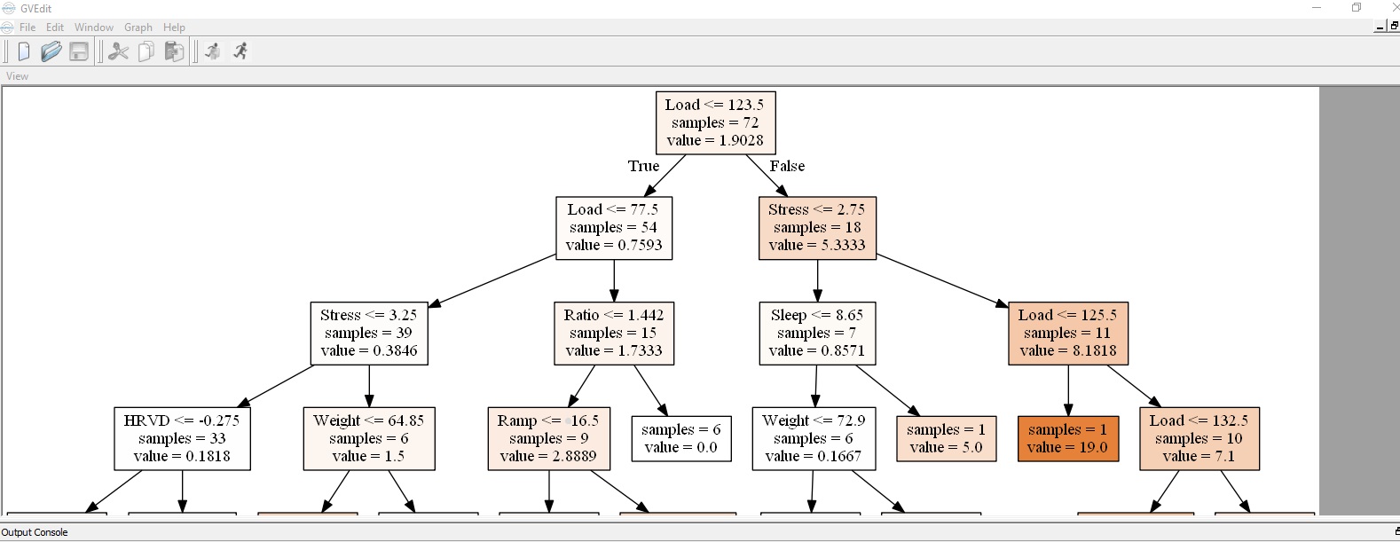
If you follow the different sides of the tree you can see the extremes…

Right side of tree (Injured) – Average training load greater than 123.5TSS/d (18 athletes), stress levels greater than 2.75 (11 of the 18) = very good chance of injury!

Left side of tree (Not injured) – Load less than 123.5 (54 athletes), load less than 77.5 (39 of the 54), average stress levels less than 3.25 (33 of the 39) & HRV (lnRMSSD) within 0.275 of your mean = healthy athlete!

Of course, left side also equals non-competitive athlete (at those training loads :-) so for an athlete also serious about performance, they’ll be hovering in the middle – hopefully back and forth in accordance with life stress! And there may be another tree in the proverbial forest that the coach and athlete are also keeping in view – a performance tree! Actually you may want to also 'plant' a sickness tree & a training response tree, but you get my drift! :-)

The appeal of this sort of model to a coach (or the 'if-then' mind of a computer programmer :-) is obvious. Fundamentally coaching is a decision making process where the coach is weighing a bunch of input variables to determine the appropriate course of action. The machine can help the coach visualize the weighting of these variables so that the coach & athlete can make more informed decisions and see very clearly which branch of the decision tree they are heading down - the safety & enjoyment of an injury free season or the peril & heartache of a season-ending injury.

While a simple...

.... is hardly revolutionary programming (in either a computer or coaching sense!), this analysis shows that something as basic as this little 'check in' can significantly decrease the chance of injury among the group. Furthermore, it can funnel the information coming to the coach from a large number of athletes so that the coach is more aware of the athletes that may require further attention/investigation via more traditional routes - "Bob, I saw you noted that you were under a bit of stress today?".

Simply, enlisting the help of our machine friends can augment the coach & athletes ability to...

Train smart,

AC

  Tweet